Real World Algorithms

While we use algorithms to solve problems with computers, these problems are not limited to computer science. Moreover, often the same algorithm may find applications in very different areas. For example, graphs are used to represent networks, but there is no a-priori limitation on what kind of networks these may be. We can use graphs for computer networks, road networks, electricity distribution networks, or social networks.

Zeroing in on social networks, we can use them to study the spread of a disease, as disease can spread through our contacts. We can also use them to investigate how to halt the spread of a disease. If we have a network, a graph, in which we have humans connected to other humans to whom they may spread the disease, we can fight a pandemic if we detect those persons that we should vaccinate or isolate to minimize contagion.

Note that when are talking about “spread”, “pandemic”, or “contagion”, we are not necessarily referring to a biological disease. We may, for instance, be interested in stopping the transmission of fake news through a social network, or arrest the spread of a computer virus, through a computer network.

To inoculate a network is to detect those nodes, or graph vertices, that exert the maximum influence on the whole network. One possible way to do that is as follows:

1. We find the vertex with the greatest number of links; that is, the vertex with the highest degree. If there are more than one vertices with the same, maximum number of links, we may break the tie using any rule we want; if vertices are numbered arithmetically, we may pick the smallest numbered vertex.

2. We vaccinate, or isolate, that vertex. In reality, we take it out of the graph, as this will ensure that nothing will be spread through that node any more.

3. We go back to step 1.

We repeat steps 1–3 for as many nodes as we want.

In the following figures you can see the process of removing four nodes, selecting each time the node with the highest degree. The nodes that we remove are painted white, while we use different colors or the connected components of the graph.

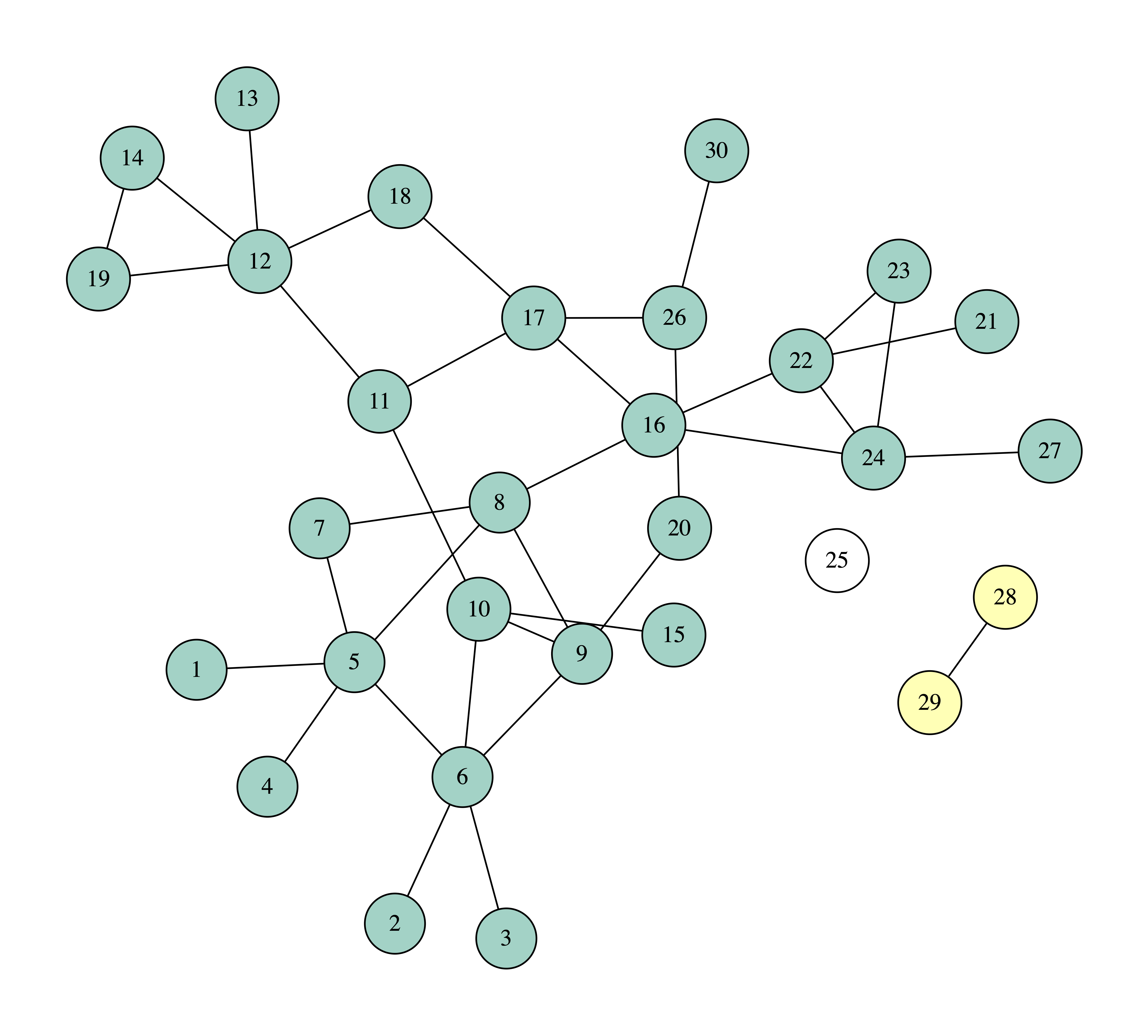
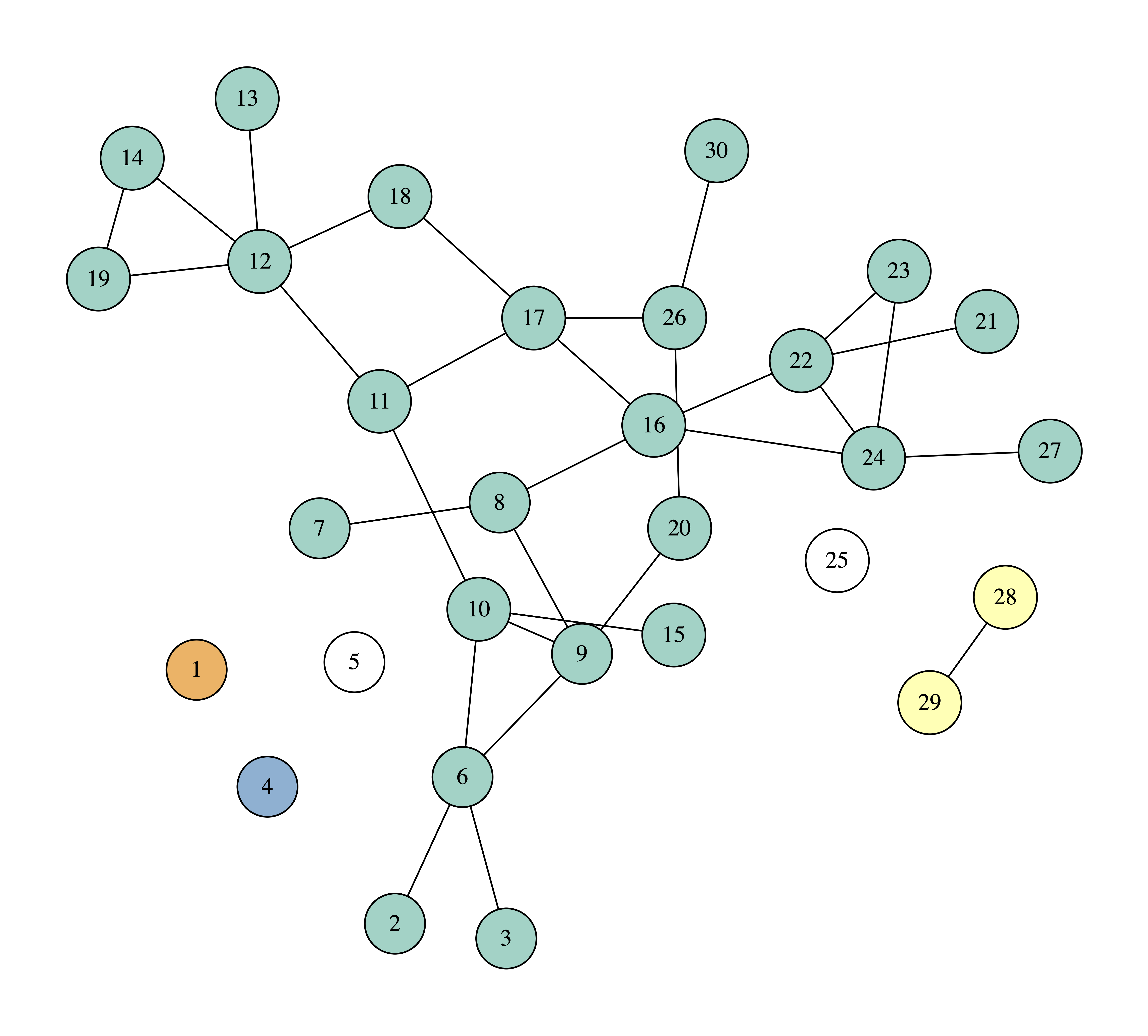
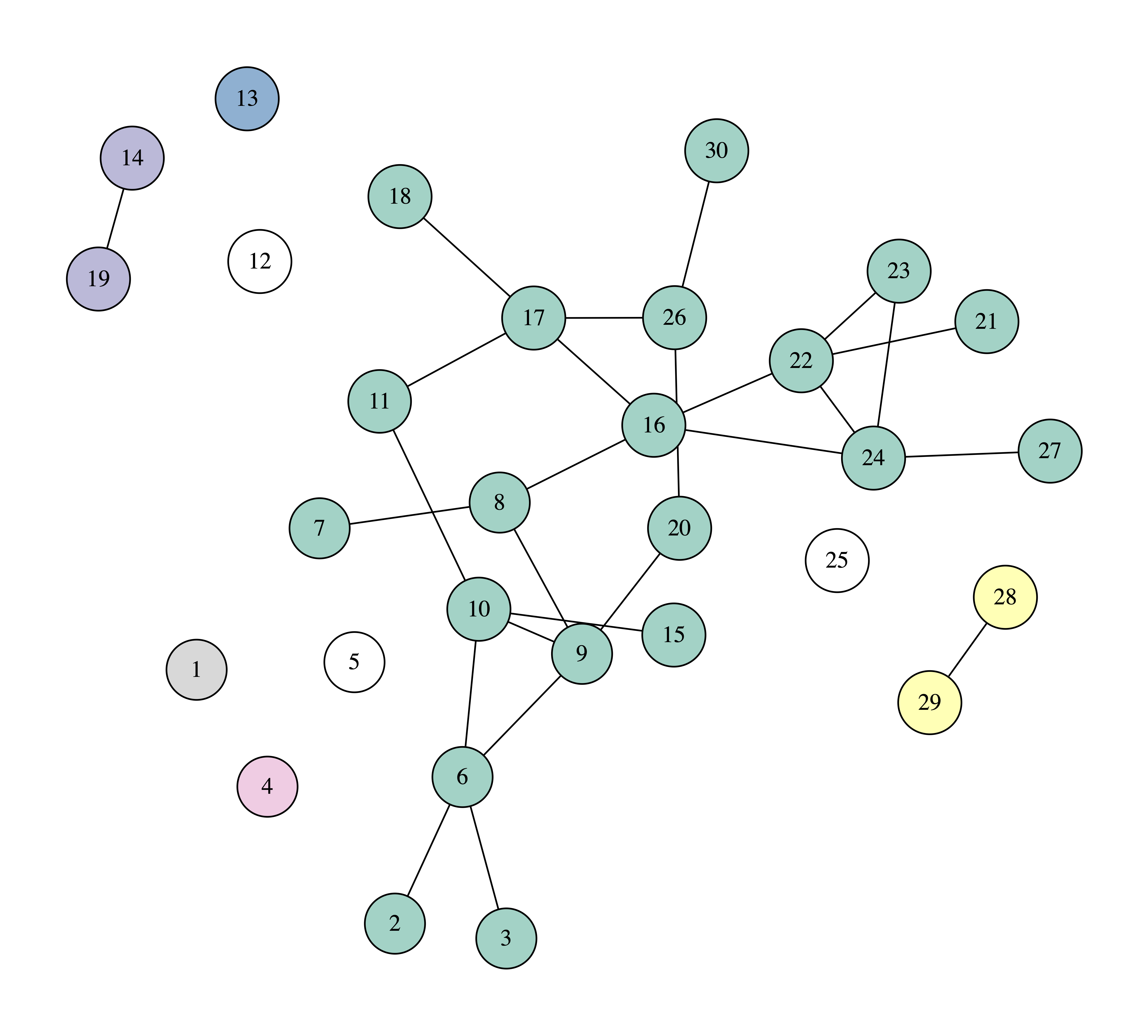
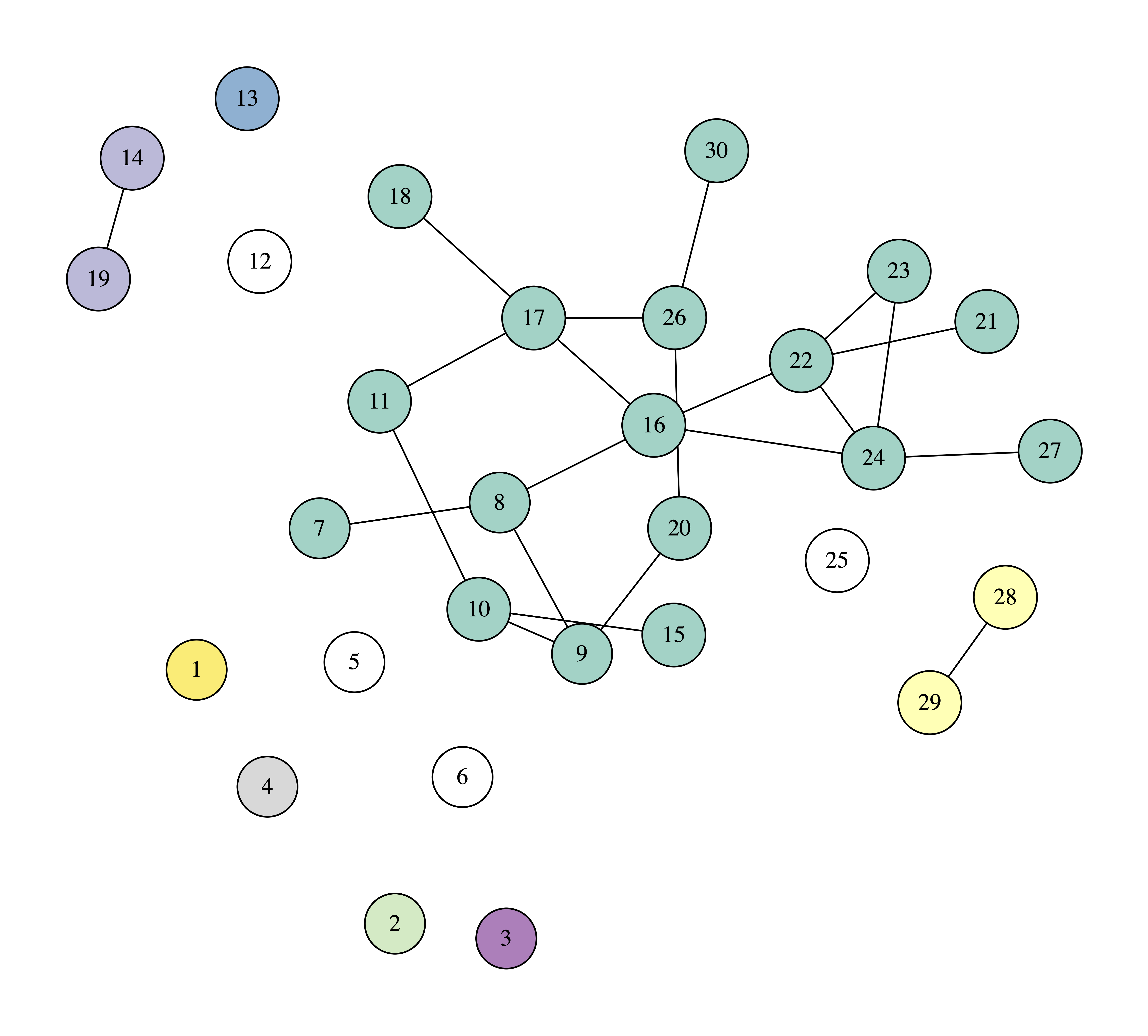
We can observe that after removing four nodes the biggest connected component consists of 17 nodes, which means that if one becomes sick, the disease will spread to another 16 nodes.

In many networks a different way of going about the problem is more efficient. Instead of taking as the node with the greatest influence the one that has the largest degree, we define the collective influence of a node as follows:

$$ \mathrm{CI}(i, r) = (k_i -1) \sum_{j \in \vartheta\mathrm{Ball}(i, r)} (k_j - 1) $$

In this definition:

• $i$ is the node whose collective influence we are calculating and $k_i$ is the degree of node $i$.

• $\mathrm{Ball}(i, r)$ is the set of nodes whose shortest path from node $i$ does not exceed $r$. If you could draw a circle with radius $r$ links around node $i$, nodes $j$ are the nodes that would fall inside the circle. If you would prefer to talk in three dimensions, they would be the nodes that fall inside the sphere centered at node $i$ and having radius $r$.

• $\vartheta\mathrm{Ball}(i, r)$ is the set of nodes whose shortest path from node $i$ is exactly $r$. If you could draw a circle with radius $r$ links around node $i$, nodes $j$ are the nodes that fall on the perimeter of the circle. If you would prefer to talk in three dimensions, they would be the nodes that fall on the surface of the sphere centered at node $i$ and having radius $r$.

Following the above, to calculate the collective influence of a node $i$, we find the nodes whose shortest path from $i$ is equal to $r$ and we take the sum of the links of each one of them, $k_j$ for node $j$, minus one. Finally, we multiply the sum with the number of links of $i$, $k_i$, minus one.

Using the collective influence, we can now dismantle a network like this:

1. We calculate the collective influence of every node.

2. We select the node with the biggest collective influence. If there are more than one node with the same collective influence we may break the tie using any rule we want; if nodes are numbered arithmetically, we may pick the smallest numbered vertex.

3. We remove that node.

4. We update the collective influence of the nodes that are affected by the removal of the node in step 3. These are the nodes inside $\mathrm{Ball}(i, r+1)$, that is, the nodes that lie inside a circle (or a sphere) of radius $r+i$ links away from node $i$, where $i$ is the node that we removed in step 3.

5. We return to step 2.

We repeat steps 2–5 for as many nodes as we want.

To implement this algorithm we need a way to calculate $\vartheta\mathrm{Ball}(i, r)$ and $\mathrm{Ball}(i, r+1)$. In order to detect the nodes that lie inside a given distance from another note, it suffices to use a variant of breadth-first search (BFS), where, as we move further away from our starting node, we keep count of the links we travel along.

In the following images you can see how we can protect a network against contagion by taking out four nodes with the largest, at each point, collective influence, using $r = 2$. Again, we use white to paint the removed nodes, and other colors for the connected components.

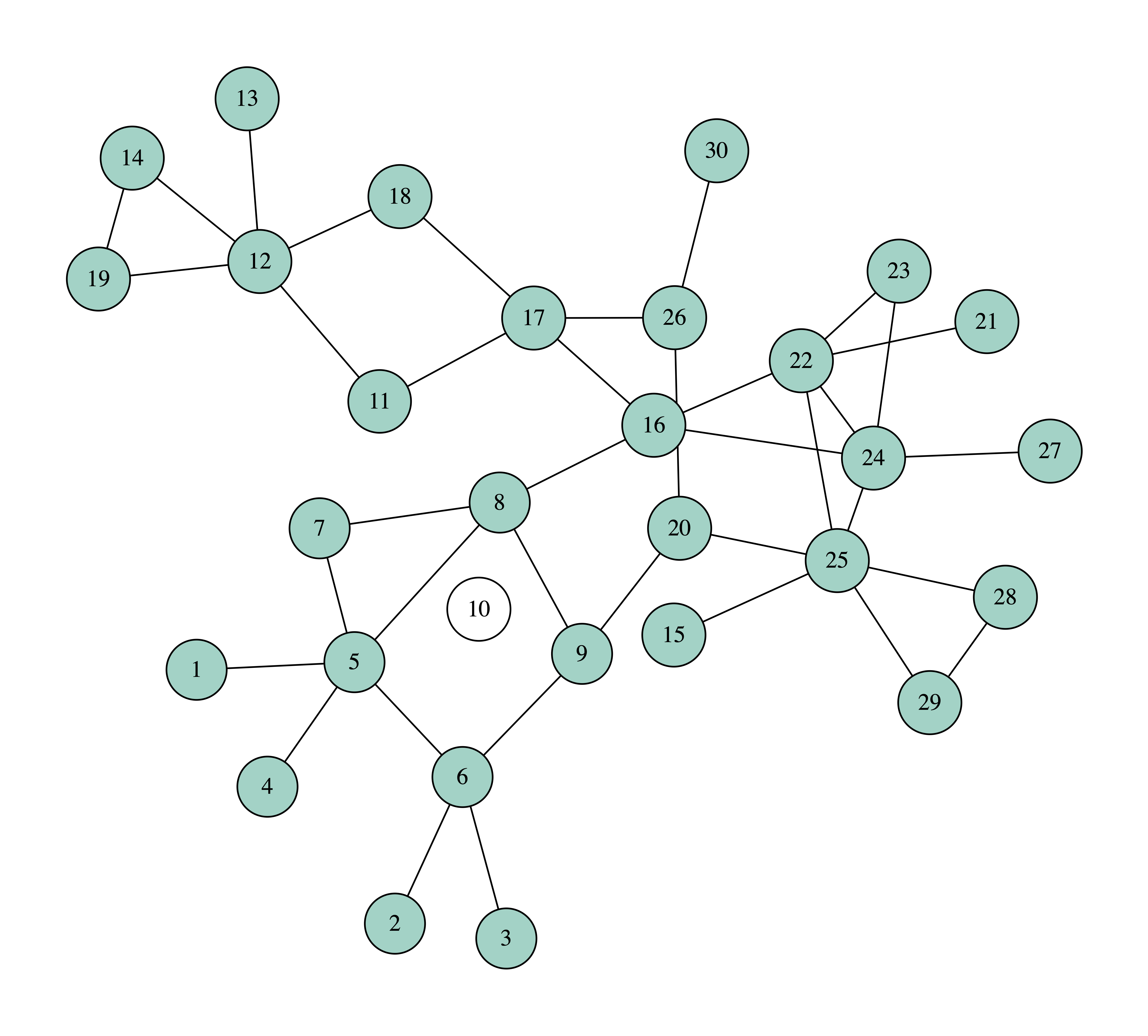
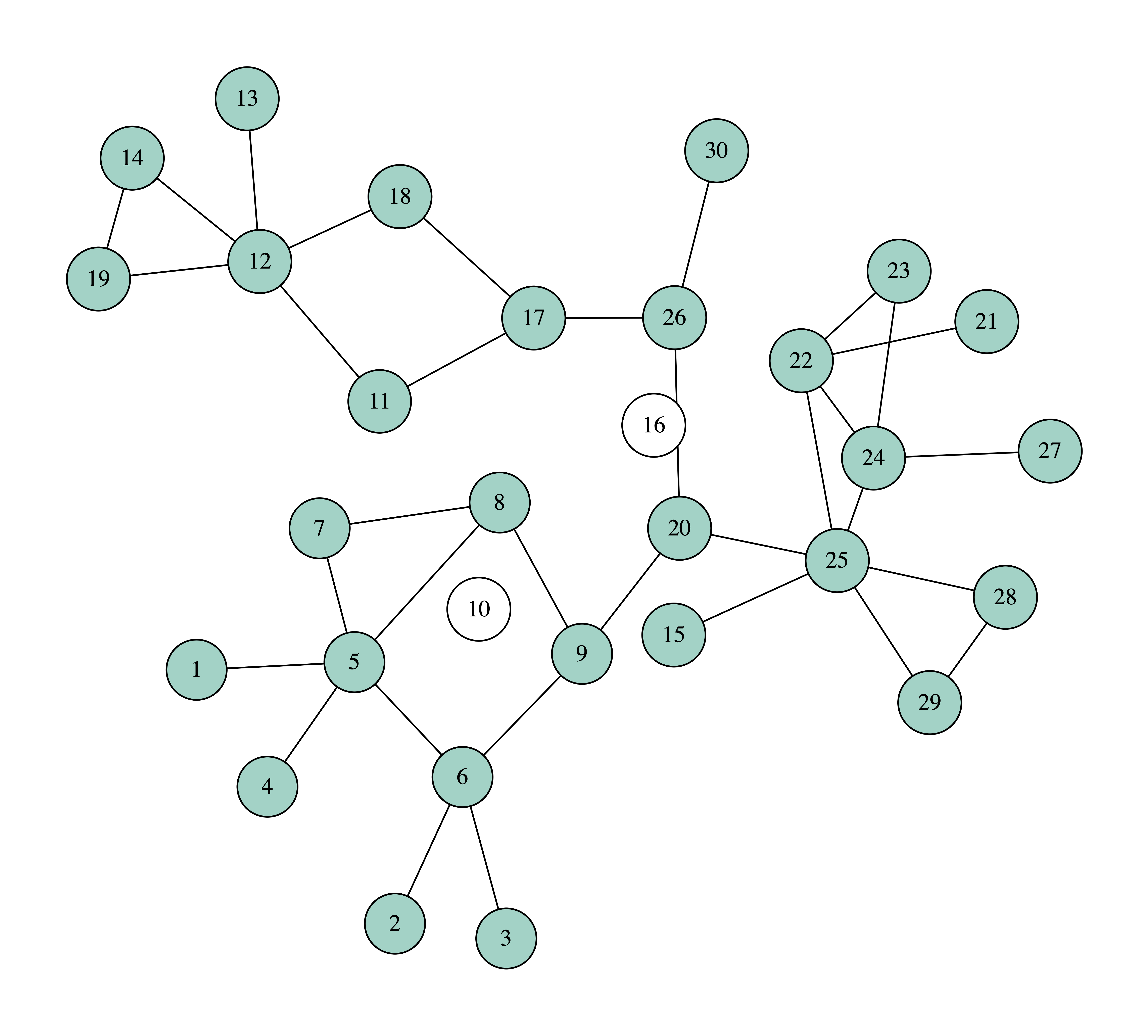
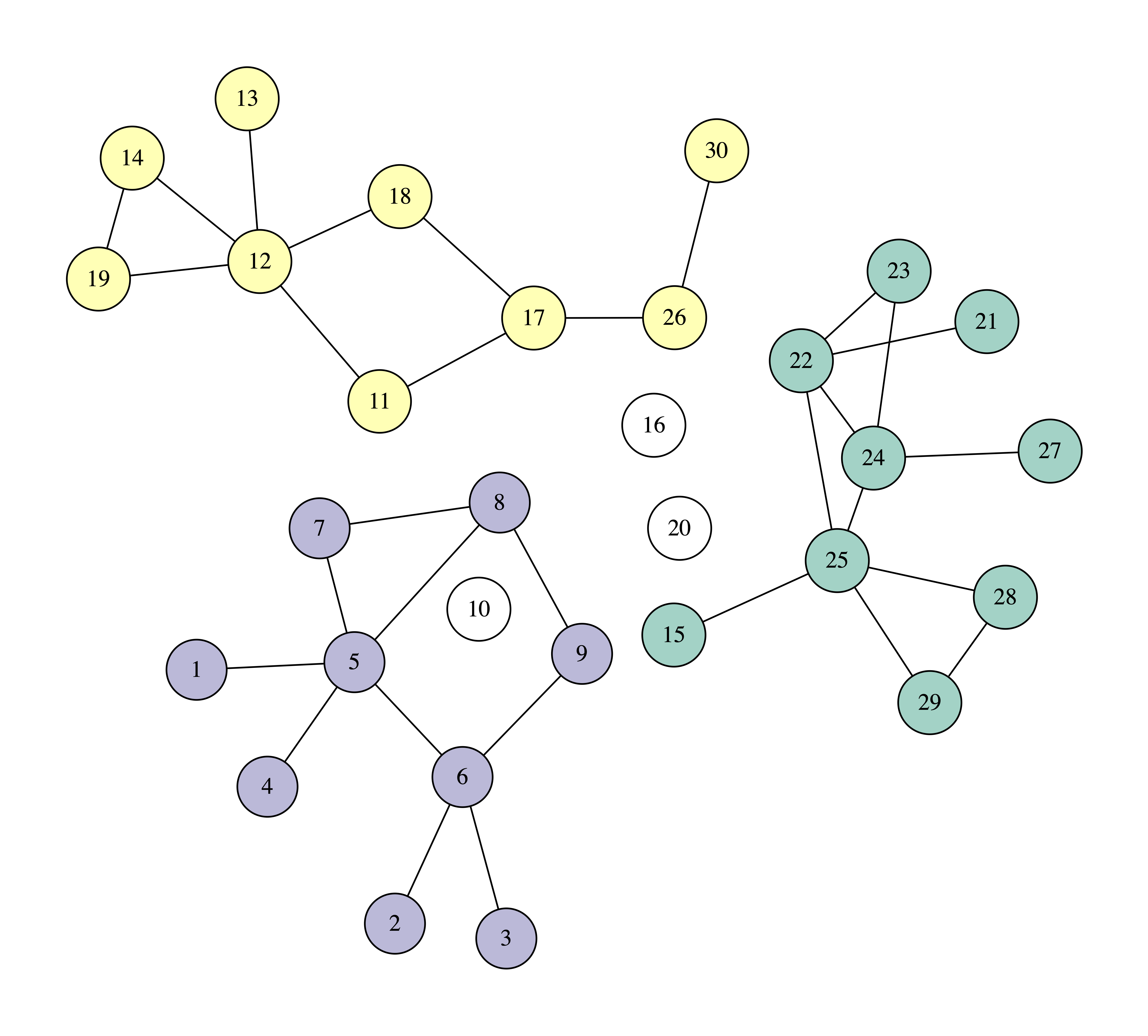
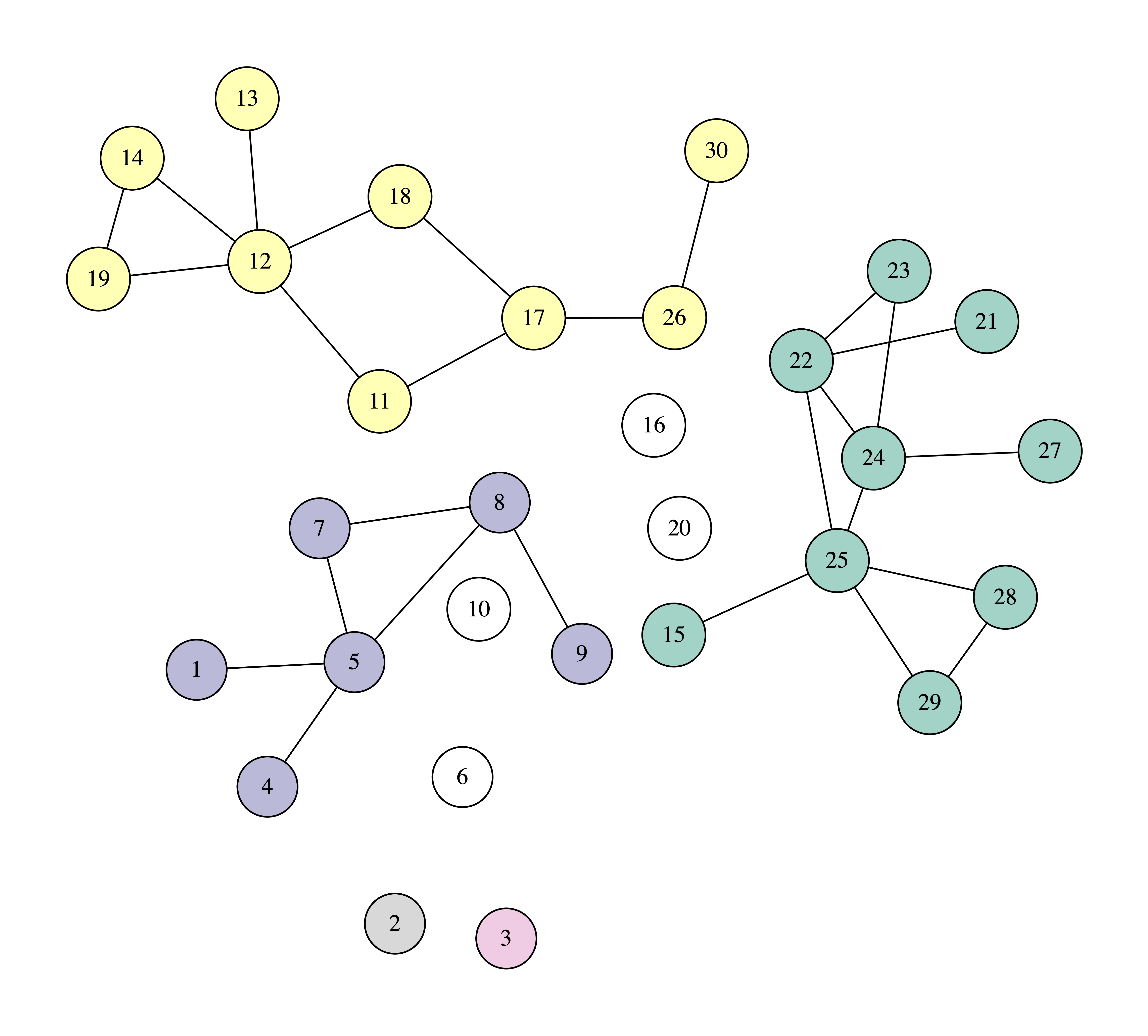
We can observe that after removing just three nodes, the biggest connected component has only nine nodes. So, with these three nodes we managed to dismantle the network more than with the four nodes using the previous method, that of selecting nodes based on their degree. In the process, node 10 is removed first, as it has the greatest collective influence, equal to 63. Verify this calculation to make sure that you have understood the definition of collective influence.

Your objective in this assignment is to write a Python program that will read a file describing a graph and then will select the nodes to remove using both of the above ways.

Requirements

You will write a program called network-destruction.py. You may use the standard Python libraries argparse and sys, but not any others. Your program will be called as follows:

python network_destruction.py [-d] [-r RADIUS] num_nodes input_file

The meaning of the program arguments is:

• -d: optional argument; if given,the program will use the degree of each node and not its collective influence. That is, it will operate as in the first example we saw. Otherwise, it will operate using the collective influence, as in the second example.

• -r RADIUS: optional argument; the program will use the value RADIUS for $r$, or will default to $r = 2$ otherwise.

• num_nodes: the number of nodes to remove; mandatory argument.

• input_file: the name of the file describing the graph.

The file indicated by input_file will have the format:

1 2
1 3
2 4
...

that is, it will consist of lines, each one containing two numbers. If the two numbers are x and y, the graph will have a link between x and y. The graph is undirected, so we can take it as granted that it will also have the opposite link, from y to x. The nodes will always be numbers, starting from $1$ and increasing by one: $1$, $2$, $\ldots$.

The program will about a sequence of lines; each line will contain the node that is removed and its metric.

Examples

Example 1

If we use the example file destruction_example_1.txt:

python network_destruction.py -r 2 4 destruction_example_1.txt

we will get:

10 63
16 51
20 30
6 9

That is, we will first take out node 10 with collective influece 63, then node 16 with collective influence 51, and so on.

If we use the example file destruction_example_1.txt as:

python network_destruction.py -d 4 destruction_example_1.txt

we will get:

25 6
5 5
12 5
6 4

This time we first take out node 25 with degree 6, then node 5 with degree 5, and so on.

Example 2

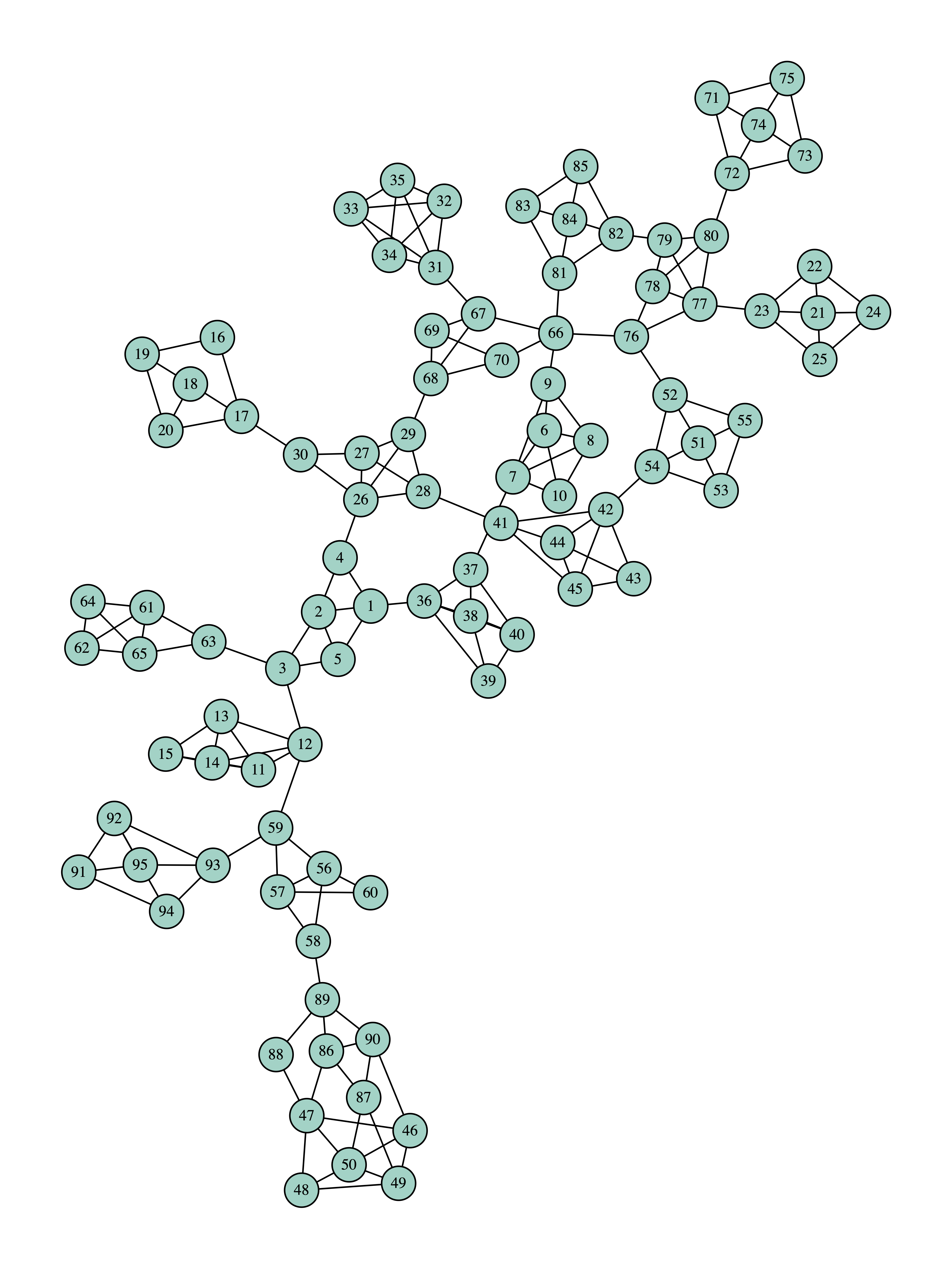
If we use the example file destruction_example_2.txt with:

python network_destruction.py -d 6 destruction_example_2.txt

we will get:

7 5
12 5
26 5
31 5
36 5
42 5

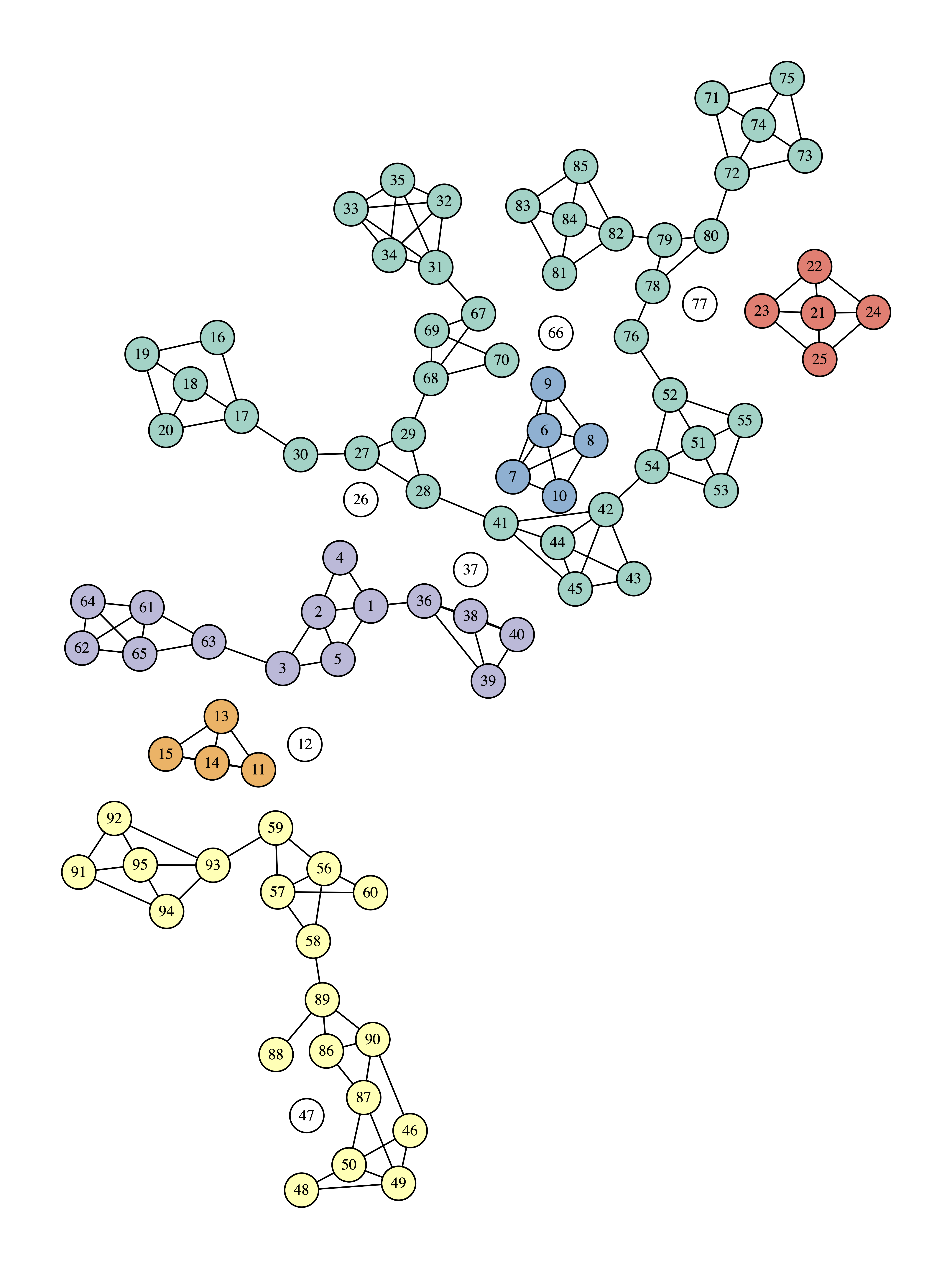
If we give:

python network_destruction.py -r 2 6 destruction_example_2.txt

we will get:

66 148
12 72
77 64
26 60
47 48
37 45

The initial graph is:

The final graph is:

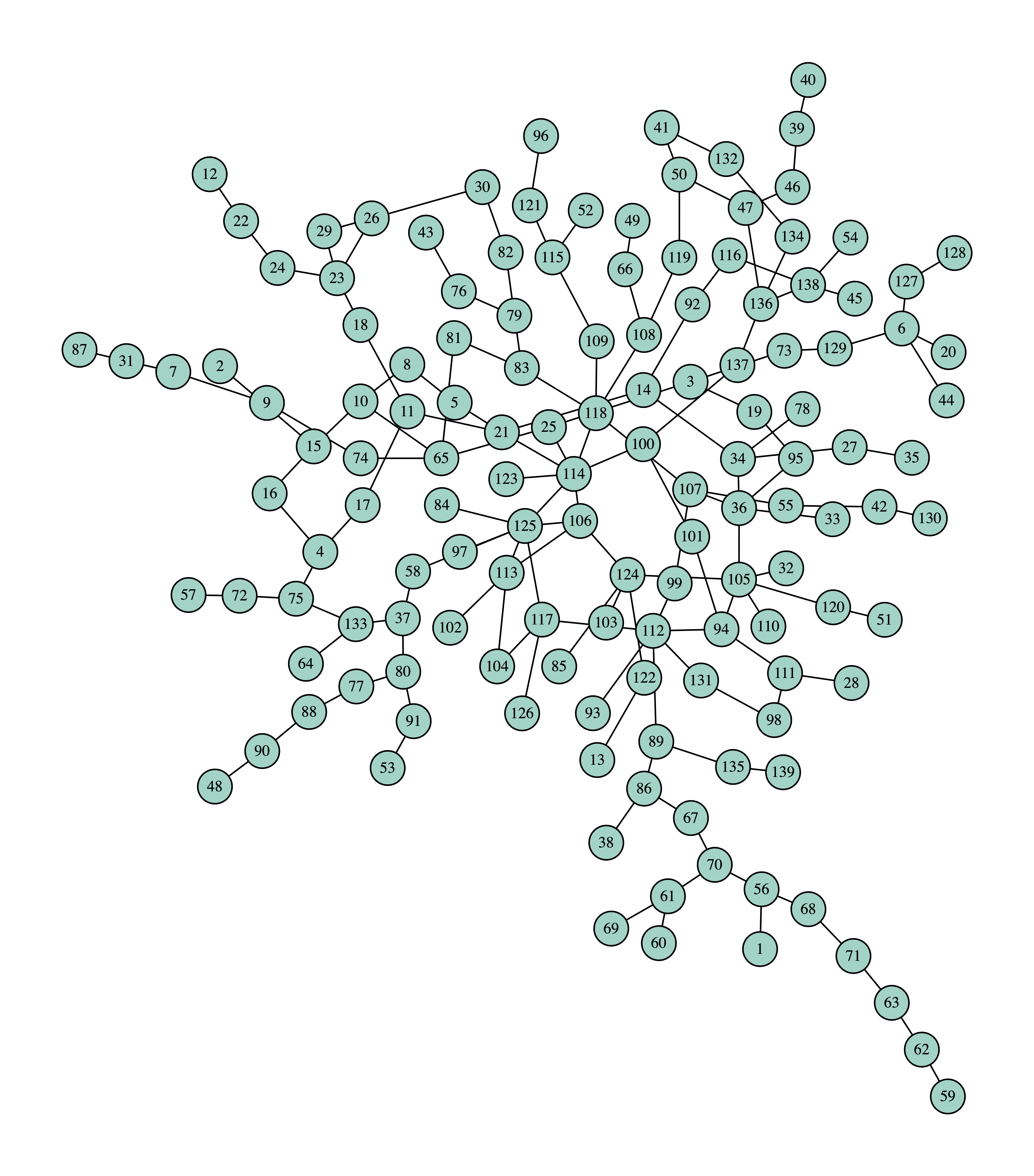
Example 3

If we use the example file destruction_example_3.txt with:

python network_destruction.py -c 10 destruction_example_3.txt

we will get:

114 7
105 6
112 6
125 6
6 4
23 4
34 4
65 4
107 4
124 4

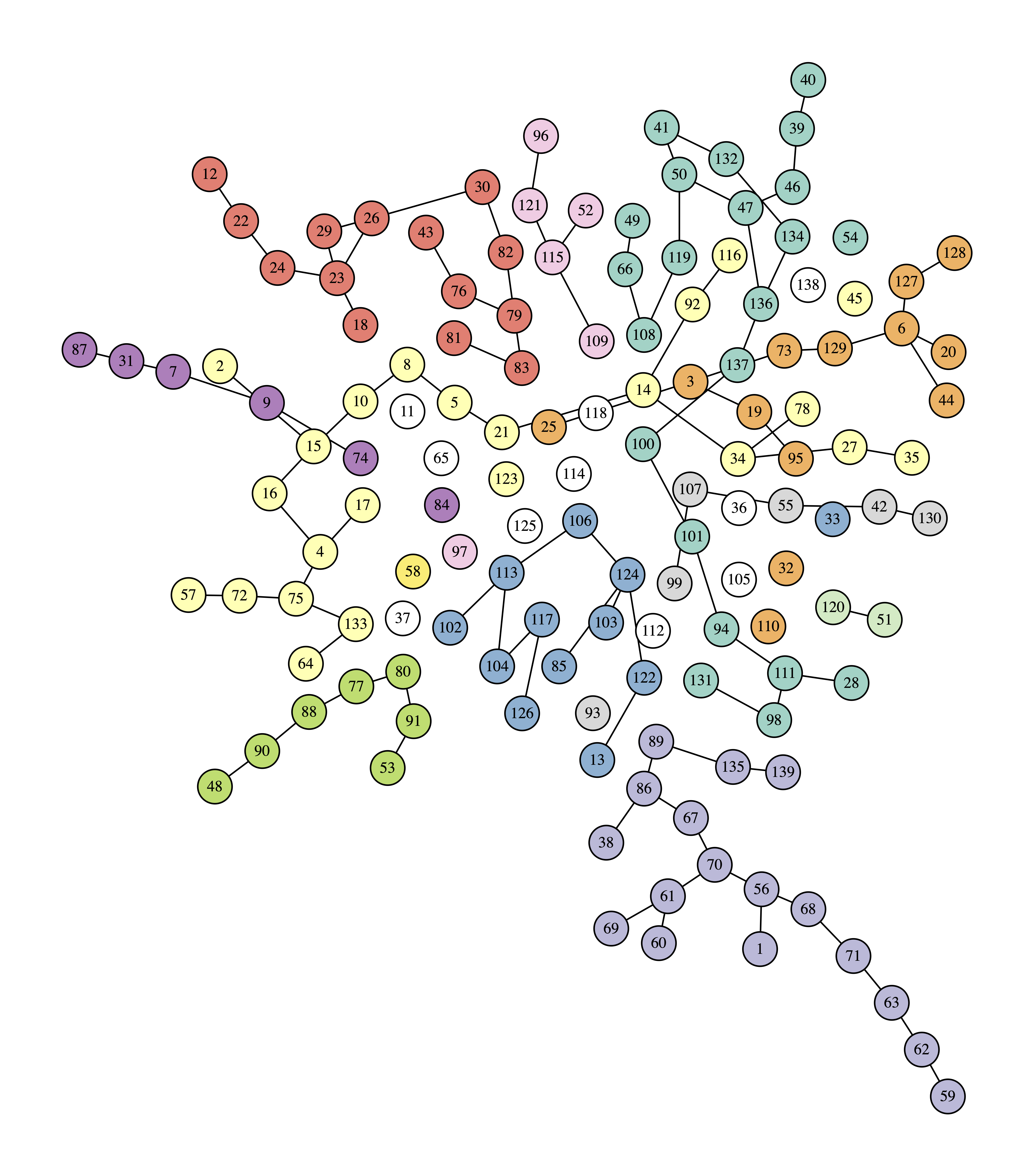
If we give:

python network_destruction.py -r 3 10 destruction_example_3.txt

we will get:

114 270
105 125
112 75
118 39
125 25
11 24
65 21
138 21
36 15
37 8

The initial graph is:

The final graph is:

Optionally

To get a better understanding of how the algorithm works, a good idea is to add another switch to the program, -t (for trace), which will display the connected components after each node removal.

Having done that, you can visualize the evolution by adding functionality to produce a series of images like the ones you have seen here. To create them you can use graphviz through its Python interface.

Notes

For an overview of network destruction using collective influence, see [1]. The algorithm was presented in [2]. For details on its implementation, see [3].

Bibliography

- István A. Kovács and Albert-László Barabási. Destruction perfected. Nature, 524(7563):38–39, 2015. doi:10.1038/524038a. ↩
- Flaviano Morone and Hernán A. Makse. Destruction perfected. Nature, 524(7563):65–68, 2015. doi:10.1038/nature14604. ↩
- Flaviano Morone, Byungjoon Min, Lin Bo, Romain Mari, and Hernán A. Makse. Collective influence algorithm to find influencers via optimal percolation in massively large social media. Scientific Reports, 2016. doi:10.1038/srep30062. ↩