Real World Algorithms

We can carry out various calculations on matrices, like for instance multiplying them. Apart from traditional matrix multiplication, we can also define boolean matrix multiplication when our matrices are boolean, that is, when their elements are ones and zeros. To see what exactly boolean matrix multiplication is, let us start from plain matrix multiplication.

If we have a matrix $A$ with dimensions $n \times m$:

$$A ={\begin{pmatrix}a_{11} & a_{12}& \cdots &a_{1m}\ a_{21} & a_{22} & \cdots & a_{2m} \ \vdots &\vdots & \ddots &\vdots \ a_{n1} & a_{n2}& \cdots &a_{nm}\\end{pmatrix}}$$

and a matrix $B$ with dimensions $m \times p$:

$$B ={\begin{pmatrix}b_{11} & b_{12} & \cdots & b_{1p}\ b_{21} & b_{22} & \cdots &b_{2p}\ \vdots &\vdots & \ddots &\vdots \ b_{m1} & b_{m2} & \cdots &B_{mp}\ \end{pmatrix}}$$

then their product is matrix $C$, with dimensions $n \times p$:

$$C ={\begin{pmatrix} c_{11} & c_{12} & \cdots & c_{1p}\ c_{21} & c_{22} & \cdots & c_{2p}\ \vdots & \vdots & \ddots & \vdots \ c_{n1} & c_{n2} & \cdots & c_{np}\\end{pmatrix}}$$

In this matrix, each element $c_{ij}$ is the result of the sum of the products of every element of line $i$ with the corresponding element of column $j$:

$$c_{ij}=\sum {k=1}^{m}a$$}b_{kj

To perform the calculations for all elements of $C$ we need time $O(n^3)$ if we apply the above formula.

Now, if we have binary numbers, we can define boolean multiplication as the following operation, which is equivalent to the logical AND operation, also called conjunction, whose symbol is $\wedge$:

$$ \begin{align} 1 \wedge 1 = 1 \times 1 = 1\ 1 \wedge 0 = 1 \times 0 = 0\ 0 \wedge 1 = 0 \times 1 = 0\ 0 \wedge 0 = 0 \times 0 = 0\ \end{align} $$

Along the same lines we can define boolean addition as the following operation, equivalent to the logical OR operation, also called disjunction, whose symbol is $\vee$:

$$\begin{align} 1 \vee 1 = 1 + 1 = 1\ 1 \vee 0 = 1 + 0 = 1\ 0 \vee 1 = 0 + 1 = 1\ 0 \vee 0 = 0 + 0 = 0\ \end{align}$$

Once we have defined boolean multiplication and boolean addition, we can define boolean matrix multiplication, where each element $c_{ij}$ is defined as before, but using boolean operations:

$$c_{ij}= \bigvee {k=1}^{m}a$$} \wedge b_{kj

For example, if we have

$$A ={\begin{bmatrix} 1 & 1 & 0 & 0 & 0 \ 0 & 0 & 1 & 1 & 1 \ 1 & 0 & 0 & 1 & 0 \ 1 & 0 & 0 & 1 & 1 \ 1 & 0 & 1 & 0 & 1\ \end{bmatrix}}$$

$$B ={\begin{bmatrix} 0 & 1 & 0 & 0 & 1 \ 0 & 0 & 0 & 0 & 0 \ 1 & 1 & 0 & 0 & 1 \ 1 & 0 & 1 & 0 & 0 \ 1 & 1 & 0 & 1 & 0\ \end{bmatrix}}$$

then their boolean product is the matrix:

$$C ={\begin{bmatrix} 0 & 1 & 0 & 0 & 1 \ 1 & 1 & 1 & 1 & 1 \ 1 & 1 & 1 & 0 & 1 \ 1 & 1 & 1 & 1 & 1 \ 1 & 1 & 0 & 1 & 1\ \end{bmatrix}}$$

To calculate the boolean product we can perform the calculations as we described them. We can do something different, though, which is our objective here. In particular, we will use the four Russians algorithm[2], as described in section 6.6 of [1]. In what follows, we will assume that the two matrices $A$ and $B$ have dimensions $n \times n$.

We start by partitioning the two matrices in $\lceil{n / \lg n}\rceil$ pieces, the $A$ matrix column-wise and the $B$ matrix row-wise:

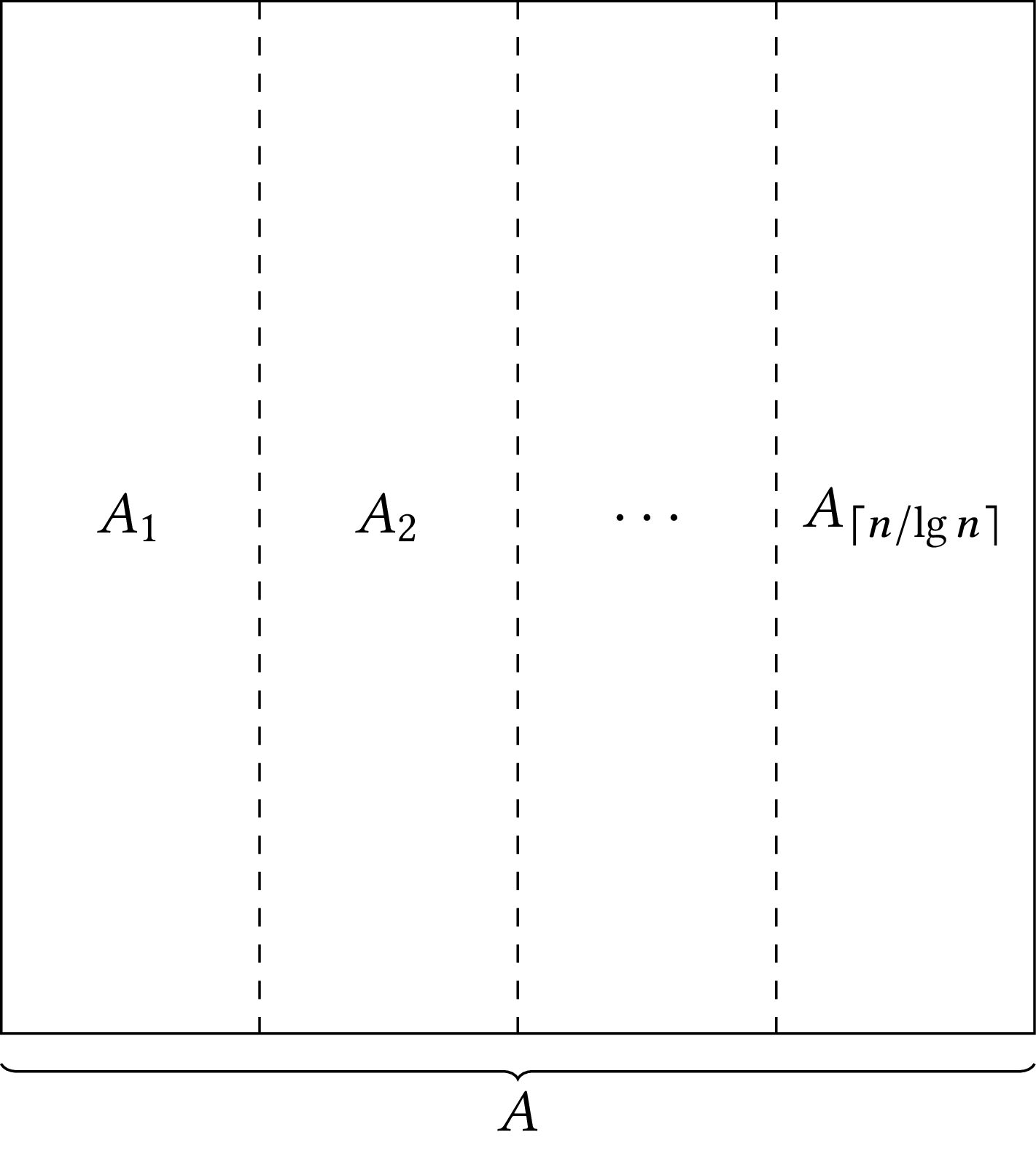
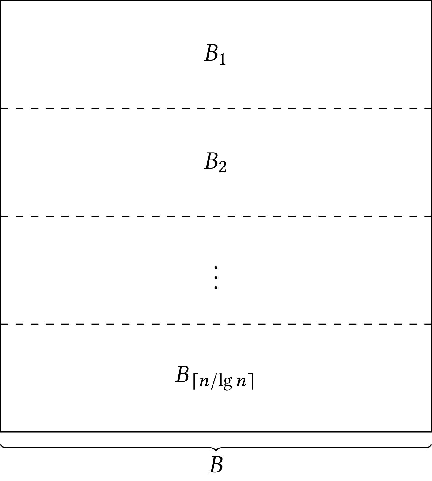
That means that each piece of $A$ will have dimensions $n \times \lfloor{\lg n}\rfloor$ and each piece of $B$ will have dimensions $\lfloor{\lg n}\rfloor \times n$. If $n$ is not divided by $\lg n$, we pad the last part of $A$ with zero columns and the last part of $B$ with zero rows.

Now note that if we have two matrices $Α$ and $B$, not necessarily boolean, with dimensions $n\times n$, and we partition them as we described, their product $AB$ can be derived by taking the products of the parts $A_i \times B_i$ and sum everything together:

$$ A B = \sum {i=1}^{\lceil{n / \lg n}\rceil}A$$}B_{i

You can verify that each of $A_i B_i$ is a matrix with dimensions $n \times n$.

In our example, we have:

$$A_1 ={\begin{bmatrix} 1 & 1 \ 0 & 0 \ 1 & 0 \ 1 & 0 \ 1 & 0 \ \end{bmatrix}}$$

and:

$$B_1 ={\begin{bmatrix} 0 & 1 & 0 & 0 & 1 \ 0 & 0 & 0 & 0 & 0 \ \end{bmatrix}}$$

so:

$$A_1 B_1 ={\begin{bmatrix} 0 & 1 & 0 & 0 & 1 \ 0 & 0 & 0 & 0 & 0 \ 0 & 1 & 0 & 0 & 1 \ 0 & 1 & 0 & 0 & 1 \ 0 & 1 & 0 & 0 & 1\ \end{bmatrix}}$$

Continuing, we have:

$$A_2 ={\begin{bmatrix} 0 & 0 \ 1 & 1 \ 0 & 1 \ 0 & 1 \ 1 & 0 \ \end{bmatrix}}$$

and:

$$B_2 ={\begin{bmatrix} 1 & 1 & 0 & 0 & 1 \ 1 & 0 & 1 & 0 & 0 \ \end{bmatrix}}$$

so:

$$A_2 B_2 ={\begin{bmatrix} 0 & 0 & 0 & 0 & 0 \ 1 & 1 & 1 & 0 & 1 \ 1 & 0 & 1 & 0 & 0 \ 1 & 0 & 1 & 0 & 0 \ 1 & 1 & 0 & 0 & 1 \end{bmatrix}}$$

Finally, we have:

$$A_3 ={\begin{bmatrix} 0 & 0 \ 1 & 0 \ 0 & 0 \ 1 & 0 \ 1 & 0 \ \end{bmatrix}}$$

and:

$$B_3 ={\begin{bmatrix} 1 & 1 & 0 & 1 & 0 \ 0 & 0 & 0 & 0 & 0 \ \end{bmatrix}}$$

so:

$$A_3 B_3 ={\begin{bmatrix} 0 & 0 & 0 & 0 & 0 \ 1 & 1 & 0 & 1 & 0 \ 0 & 0 & 0 & 0 & 0 \ 1 & 1 & 0 & 1 & 0 \ 1 & 1 & 0 & 1 & 0 \end{bmatrix}}$$

If we take the boolean sum of the products, we get:

$$A_1 B_1 + A_2 B_2 + A_3 B_3 = {\begin{bmatrix} 0 & 1 & 0 & 0 & 1 \ 0 & 0 & 0 & 0 & 0 \ 0 & 1 & 0 & 0 & 1 \ 0 & 1 & 0 & 0 & 1 \ 0 & 1 & 0 & 0 & 1\ \end{bmatrix}} + {\begin{bmatrix} 0 & 0 & 0 & 0 & 0 \ 1 & 1 & 1 & 0 & 1 \ 1 & 0 & 1 & 0 & 0 \ 1 & 0 & 1 & 0 & 0 \ 1 & 1 & 0 & 0 & 1 \end{bmatrix}} + {\begin{bmatrix} 0 & 0 & 0 & 0 & 0 \ 1 & 1 & 0 & 1 & 0 \ 0 & 0 & 0 & 0 & 0 \ 0 & 0 & 0 & 0 & 0 \ 1 & 1 & 0 & 1 & 0 \end{bmatrix}} = {\begin{bmatrix} 0 & 1 & 0 & 0 & 1 \ 1 & 1 & 1 & 1 & 1 \ 1 & 1 & 1 & 0 & 1 \ 1 & 1 & 1 & 1 & 1 \ 1 & 1 & 0 & 1 & 1 \end{bmatrix}}$$

which is the same result as the one we got before.

Let us focus on how we can calculate $A_i B_i$, taking as example $A_2 B_2$:

• The first row of $A_2 B_2$ is the result of taking none of the rows of $B_2$.
• The second row of $A_2 B_2$ is the result of the addition of the two rows of $B_2$.
• The third row of $A_2 B_2$ is the second row of $B_2$.
• The fourth row of $A_2 B_2$ is the second row of $B_2$.
• The fifth row of $A_2 B_2$ is the first row of $B_2$.

Therefore, each row of $A_2 B_2$ is the result of taking the boolean sum of those rows of $B_2$ for which the elements of the corresponding row of $A$ is equal to one. This holds in general. Suppose that:

$$A_i = {\begin{bmatrix} 0 & 1 & 0 \ 0 & 0 & 0 \ 1 & 1 & 0 \ 0 & 0 & 1 \ 1 & 0 & 0 \ 1 & 0 & 1 \ 1 & 1 & 1 \ 0 & 1 & 1 \ \end{bmatrix}} $$

and:

$$ B_i = {\begin{bmatrix} 0 & 1 & 1 & 0 & 1 & 0 & 0 & 1 \ 1 & 1 & 0 & 0 & 1 & 1 & 0 & 1 \ 0 & 1 & 0 & 0 & 0 & 1 & 0 & 0 \ \end{bmatrix}} $$

then:

$$A_i B_i = {\begin{bmatrix} 1 & 1 & 0 & 0 & 1 & 1 & 0 & 1 \ 0 & 0 & 0 & 0 & 0 & 0 & 0 & 0 \ 1 & 1 & 1 & 0 & 1 & 1 & 0 & 1 \ 0 & 1 & 0 & 0 & 0 & 1 & 0 & 0 \ 0 & 1 & 1 & 0 & 1 & 0 & 0 & 1 \ 0 & 1 & 1 & 0 & 1 & 1 & 0 & 1 \ 1 & 1 & 1 & 0 & 1 & 1 & 0 & 1 \ 1 & 1 & 0 & 0 & 1 & 1 & 0 & 1 \end{bmatrix}} $$

We can see that:

• The first row of $A_i B_i$ is equal to the second row of $B_i$, as indicated by the first row of $A_i$.
• The second row of $A_i B_i$ is equal to zero, as indicated by the second row of $A_i$.
• The third row of $A_i B_i$ is equal to the boolean sum of the first and the second rows of $B_i$, as indicated by the third row of $A_i$.
• And so on for the remaining lines; e.g., the seventh row of $A_i B_i$ is equal to the boolean sum of all the rows of $B_i$.

This leads to an idea for speeding up our calculations. Since each row of the products $A_i B_i$ is the boolean sum of some rows of $B_i$, we can pre-compute all possible boolean sums of rows of $B_i$ and use each time the sum indicated by the corresponding row of $A_i$. In this way we arrive at the following algorithm:

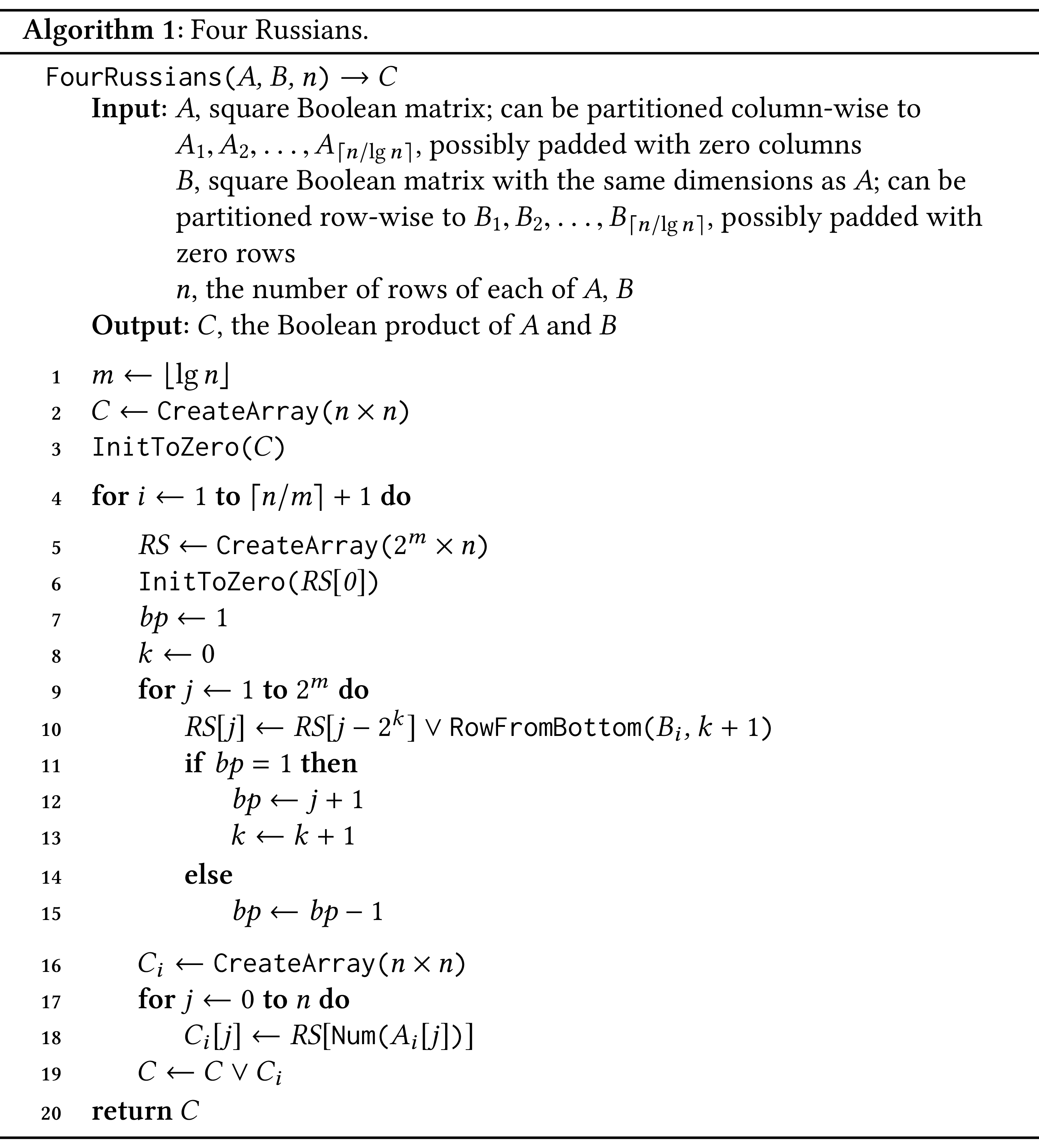
In lines 1–3 we calculate $\lfloor{\lg n}\rfloor$ and we initialize matrix $C$, which will contain the result of the multiplication. The function $\texttt{InitΤοZero(}M\texttt{)}$ initializes its argument to zero.

In each iteration of the loop of lines 4–19 we calculate a product $C_i = A_i B_i$ and we add it in $C$. Lines 5–15 calculate all possible sums of rows of $B_i$ and store them in matrix $\mathit{RS}$ (rowsums), with dimensions $2^m \times n$. To do that, we start from $\mathit{RS}[0]$, which is equal to a zero vector, and we proceed by adding to the previous sums rows from matrix $B_i$. The call $\texttt{RowFromBottom(}B_{i}, k + 1\texttt{)}$ returns the $k+1$ row counting from the end of matrix $B_i$. Lines 9–15 add rows from $B_i$ to $\mathit{RS}[j - 2^k]$, which is a sum that has already been calculated, so that we get new sums. We use a variable $\mathit{bp}$ (between powers) to know when to increase $k$: $\mathit{bp}$ counts how many numbers lie between two successive powers of two. Once we have calculated all possible boolean row sums and we have stored them in the $\mathit{RS}$ matrix, we calculate each $C_i = A_i B_i$, in lines 16–18. The call $\texttt{Num(}A_{i}[j]\texttt{)}$ returns the decimal number that corresponds to the $j$th row of matrix $A_i$. For example, if $A_{i}[j] = [1, 0, 1]$, $\texttt{Num(}A_{i}[j]\texttt{)}$ returns 5. Finally, we add each $C_i$ to $C$ inline 19.

Graphs give us an opportunity to see an application of boolean matrix multiplication. If $G = (V, E)$ is a directed graph, we can form the graph $G = (V, E)$ that has the same vertices as $G$ but one edge for any pair of nodes that are connected in $G$ (and not just the direct neighbors). The graph $G$ is called the transitive closure* of $G$. Suppose we have the graph:

Then, the transitive closure of $G$ is the graph $G*$:

To calculate the transitive closure of a graph we can use boolean matrix multiplication. If $A$ is the adjacency matrix of graph $G$, then $A^2 = A A$ is the adjacency matrix of the graph that we get from $G$ if we add to $G$ an edge for every pair of nodes that are connected with a path of length two. Similarly, $A^3 = A^2 A$ is the adjacency matrix of the graph that we get grom $G$ if we add to $G$ an edge for every pair of nodes that are connected with a path of length two or three. In general, $A^n = A^{n-1} A$ is the adjacency matrix of the graph we get if we add to $G$ an edge for every pair of nodes that are connected with a path of length 2, 3, $\ldots$, $n - 1$. For this to work, we assume that each node in $G$ is connected to itself, so in the adjancency matrix of $G$ we put ones down the left to right diagonal. More formally, we use as adjacency matrix the matrix $A \vee \mathbf{I}$, where $A$ is the initial adjacency matrix and $\mathbf{I}$ is the identity matrix.

In this assignment you will implement a program that finds the transitive closure of a graph using the four Russians algorithm.

Requirements

You will write a program called four_russians.py. The program will be called in two ways.

If the program is called with:

python four_russians.py <input_file_1> <input_file_2>

where <input_file_1> and <input_file_2> are the names of two files containing boolean matrices, the program will output their boolean product. For example, if the user specifies files array_1.txt and array_2.txt, the program will output:

1,0,1,1,0,1,1,0,0,0,1,0,0
1,0,1,1,1,1,1,0,1,1,1,1,0
1,1,0,0,1,0,0,0,0,0,1,0,1
1,0,0,1,1,0,1,1,1,1,1,1,1
0,1,1,1,0,0,1,0,1,1,1,1,1
1,1,1,0,1,1,1,1,1,1,1,1,1
1,1,1,1,1,1,1,1,1,0,1,1,1
1,0,1,1,1,1,1,0,1,0,1,1,0
1,1,1,1,0,1,1,1,1,1,1,1,1
1,0,1,1,0,1,1,1,1,0,1,0,1
1,1,1,1,0,0,1,0,0,0,0,0,1
1,1,0,1,1,0,1,1,1,1,1,1,1
1,1,1,1,0,1,0,1,1,0,0,1,1

If the program is called with:

python four_russians.py <input_file>

where <input_file> is the name of a file that contains a graph, the program will output the transitive closure of the graph. The input file will describe the graph by giving each edge in a line. For example, a file starting with:

0 1
1 2
2 3

specifies that node 0 is connected with node 1, node 1 is connected with node 2, and node 2 is connected to node 3.

The transitive closure will be described in the same way, with an edge per line. The lines must be output in ascending order. For example, if the program is given as input the file graph_1.txt, which corresponds to the graph we used above, we'll get the following output:

0 0
0 1
0 2
0 3
0 4
0 5
1 1
1 2
1 3
1 4
1 5
2 2
2 3
2 4
2 5
3 3
3 4
3 5
4 4
4 5
5 5

Notes

• The algorithm was first published in Russian, as "Об экономном построении транзитивного замыкания ориентированного графа", Доклады Академии Наук СССР 134 (3), 1970.
• The algorithm took its name because it was believed that its creators were Russians. However, although all of them lived in the Soviet Union, it is not certain that they were Russians.
• The algorithm is useful because it allows us to perform the boolean multiplication of two matrices in time $Ο(n^3/\lg n)$. This can be improved to $Ο(n^2/\lg n)$ if we implement it using bitwise operators, better than the $O(n^3)$ time taken if we just follow the definition of matrix multiplication.
• Beyond boolean multiplication, the underlying logic of the algorithm can be applied to the calculation of the distance between two strings, DNA sequence alignment, and cryptography. Check the Wikipedia article for more details.

Bibliography

- Alfred V. Aho, John E. Hopcroft, and Jeffrey D. Ullman. The Design and Analysis of Computer Algorithms. Addison-Wesley, Reading, MA, 1974. ↩
- V. L. Arlazarov, Y. A. Dinitz, and I. A. Kronrod, M. A. Faradzhev. On economical construction of the transitive closure of an oriented graph. Doklady Akademii Nauk SSSR, 194(3):487–488, 1970. ↩